Optimization Tutorial
Introduction
This section describes a sample run script for airfoil optimization with CMPLXFOIL. It is very similar to the MACH-Aero single point airfoil tutorial. This example uses pyOptSparse’s SLSQP optimizer because it comes with pyOptSparse, but SNOPT is recommended for more robustness, speed, and tunability.
The optimization problem solved in this script is
Getting set up
In addition to the required CMPLXFOIL packages, this script requires pygeo, multipoint, pyoptsparse, and mpi4py. The script can be found in CMPLXFOIL/examples/single_point.py.
Dissecting the optimization script
Import libraries
import os
import numpy as np
from mpi4py import MPI
from baseclasses import AeroProblem
from pygeo import DVConstraints, DVGeometryCST
from pyoptsparse import Optimization, OPT
from multipoint import multiPointSparse
from cmplxfoil import CMPLXFOIL, AnimateAirfoilOpt
Specifying parameters for the optimization
These parameters define the flight condition and initial angle of attack for the optimization.
mycl = 0.5  # lift coefficient constraint
alpha = 0.0 if mycl == 0.0 else 1.0  # initial angle of attack (zero if the target cl is zero)
mach = 0.1  # Mach number
Re = 1e6  # Reynolds number
T = 288.15  # 1976 US Standard Atmosphere temperature @ sea level (K)
Creating processor sets
Allocating sets of processors for different analyses can be helpful for multiple design points, but this is a single point optimization, so only one point is added.
MP = multiPointSparse(MPI.COMM_WORLD)
MP.addProcessorSet("cruise", nMembers=1, memberSizes=MPI.COMM_WORLD.size)
MP.createCommunicators()
Creating output directory
This section creates a directory in the run script’s directory in which to save files from the optimization.
curDir = os.path.abspath(os.path.dirname(__file__))
outputDir = os.path.join(curDir, "output")

if not os.path.exists(outputDir):
    os.mkdir(outputDir)
CMPLXFOIL solver setup
The options tell the solver to write out chordwise aerodynamic data (writeSliceFile) and the airfoil coordinates (writeCoordinates) every time it is called.
It also enables live plotting during the optimization (plotAirfoil).
Finally, it specifies the output directory to save these files.
aeroOptions = {
    "writeSolution": True,
    "writeSliceFile": True,
    "writeCoordinates": True,
    "plotAirfoil": True,
    "outputDirectory": outputDir,
}

# Create solver
CFDSolver = CMPLXFOIL(os.path.join(curDir, "naca0012.dat"), options=aeroOptions)
Other options allow the user to adjust the maximum iterations allowed to the XFOIL solver and to specify a location at which to trip the boundary layer.
Set the AeroProblem
We add angle of attack as a design variable (if the target lift coefficient is not zero) and set up the AeroProblem using given flow conditions.
ap = AeroProblem(
    name="fc",
    alpha=alpha if mycl != 0.0 else 0.0,
    mach=mach,
    reynolds=Re,
    reynoldsLength=1.0,
    T=T,
    areaRef=1.0,
    chordRef=1.0,
    evalFuncs=["cl", "cd"],
)
# Add angle of attack variable
if mycl != 0.0:
    ap.addDV("alpha", value=ap.alpha, lower=-10.0, upper=10.0, scale=1.0)
Geometric parametrization
This examples uses a class-shape transformation (CST) airfoil parameterization because it requires no additional files or other setup. Four CST parameters are added to the upper and lower surface (the class shape and chord length are other possible design variables through DVGeometryCST). The DVGeometryCST instance will set the initial design variables values by fitting them to the input dat file’s geometry.
nCoeff = 4  # number of CST coefficients on each surface
DVGeo = DVGeometryCST(os.path.join(curDir, "naca0012.dat"), numCST=nCoeff)

DVGeo.addDV("upper_shape", dvType="upper", lowerBound=-0.1, upperBound=0.5)
DVGeo.addDV("lower_shape", dvType="lower", lowerBound=-0.5, upperBound=0.1)

# Add DVGeo object to CFD solver
CFDSolver.setDVGeo(DVGeo)
Geometric constraints
In this section, we add volume, thickness, and leading edge radius constraints. They are chosen to achieve practical airfoils and to guide the optimizer away from infeasible design, such as the upper and lower surfaces crossing over each other.
DVCon = DVConstraints()
DVCon.setDVGeo(DVGeo)
DVCon.setSurface(CFDSolver.getTriangulatedMeshSurface())

# Thickness, volume, and leading edge radius constraints
le = 0.0001
wingtipSpacing = 0.1
leList = [[le, 0, wingtipSpacing], [le, 0, 1.0 - wingtipSpacing]]
teList = [[1.0 - le, 0, wingtipSpacing], [1.0 - le, 0, 1.0 - wingtipSpacing]]
DVCon.addVolumeConstraint(leList, teList, 2, 100, lower=0.85, scaled=True)
DVCon.addThicknessConstraints2D(leList, teList, 2, 100, lower=0.25, scaled=True)
le = 0.01
leList = [[le, 0, wingtipSpacing], [le, 0, 1.0 - wingtipSpacing]]
DVCon.addLERadiusConstraints(leList, 2, axis=[0, 1, 0], chordDir=[-1, 0, 0], lower=0.85, scaled=True)

fileName = os.path.join(outputDir, "constraints.dat")
DVCon.writeTecplot(fileName)
Optimization callback functions
This section defines callback functions that are used by the optimizer to get objective, constraint, and derivative information. See the MACH-Aero aerodynamic optimization tutorial for more information.
def cruiseFuncs(x):
    print(x)
    # Set design vars
    DVGeo.setDesignVars(x)
    ap.setDesignVars(x)
    # Run CFD
    CFDSolver(ap)
    # Evaluate functions
    funcs = {}
    DVCon.evalFunctions(funcs)
    CFDSolver.evalFunctions(ap, funcs)
    CFDSolver.checkSolutionFailure(ap, funcs)
    if MPI.COMM_WORLD.rank == 0:
        print("functions:")
        for key, val in funcs.items():
            if key == "DVCon1_thickness_constraints_0":
                continue
            print(f"    {key}: {val}")
    return funcs


def cruiseFuncsSens(x, funcs):
    funcsSens = {}
    DVCon.evalFunctionsSens(funcsSens)
    CFDSolver.evalFunctionsSens(ap, funcsSens)
    CFDSolver.checkAdjointFailure(ap, funcsSens)
    print("function sensitivities:")
    evalFunc = ["fc_cd", "fc_cl", "fail"]
    for var in evalFunc:
        print(f"    {var}: {funcsSens[var]}")
    return funcsSens


def objCon(funcs, printOK):
    # Assemble the objective and any additional constraints:
    funcs["obj"] = funcs[ap["cd"]]
    funcs["cl_con_" + ap.name] = funcs[ap["cl"]] - mycl
    if printOK:
        print("funcs in obj:", funcs)
    return funcs
Optimization problem
This section sets up the optimization problem by adding the necessary design variables and constraints. An additional constraint for this problem enforces that the first upper and lower surface CST coefficients are equal. This is to maintain continuity on the leading edge. It also prints out some useful information about the optimization problem setup. See the MACH-Aero aerodynamic optimization tutorial for more information.
# Create optimization problem
optProb = Optimization("opt", MP.obj)

# Add objective
optProb.addObj("obj", scale=1e4)

# Add variables from the AeroProblem
ap.addVariablesPyOpt(optProb)

# Add DVGeo variables
DVGeo.addVariablesPyOpt(optProb)

# Add constraints
DVCon.addConstraintsPyOpt(optProb)

# Add cl constraint
optProb.addCon("cl_con_" + ap.name, lower=0.0, upper=0.0, scale=1.0)

# Enforce first upper and lower CST coefficients to add to zero
# to maintain continuity at the leading edge
jac = np.zeros((1, nCoeff), dtype=float)
jac[0, 0] = 1.0
optProb.addCon(
    "first_cst_coeff_match",
    lower=0.0,
    upper=0.0,
    linear=True,
    wrt=["upper_shape", "lower_shape"],
    jac={"upper_shape": jac, "lower_shape": jac},
)

# The MP object needs the 'obj' and 'sens' function for each proc set,
# the optimization problem and what the objcon function is:
MP.setProcSetObjFunc("cruise", cruiseFuncs)
MP.setProcSetSensFunc("cruise", cruiseFuncsSens)
MP.setObjCon(objCon)
MP.setOptProb(optProb)
optProb.printSparsity()
optProb.getDVConIndex()
Run optimization
Run the optimization using pyOptSparse’s SLSQP optimizer and print the solution.
# Run optimization
optOptions = {"IFILE": os.path.join(outputDir, "SLSQP.out")}
opt = OPT("SLSQP", options=optOptions)
sol = opt(optProb, MP.sens, storeHistory=os.path.join(outputDir, "opt.hst"))
if MPI.COMM_WORLD.rank == 0:
    print(sol)
Postprocessing
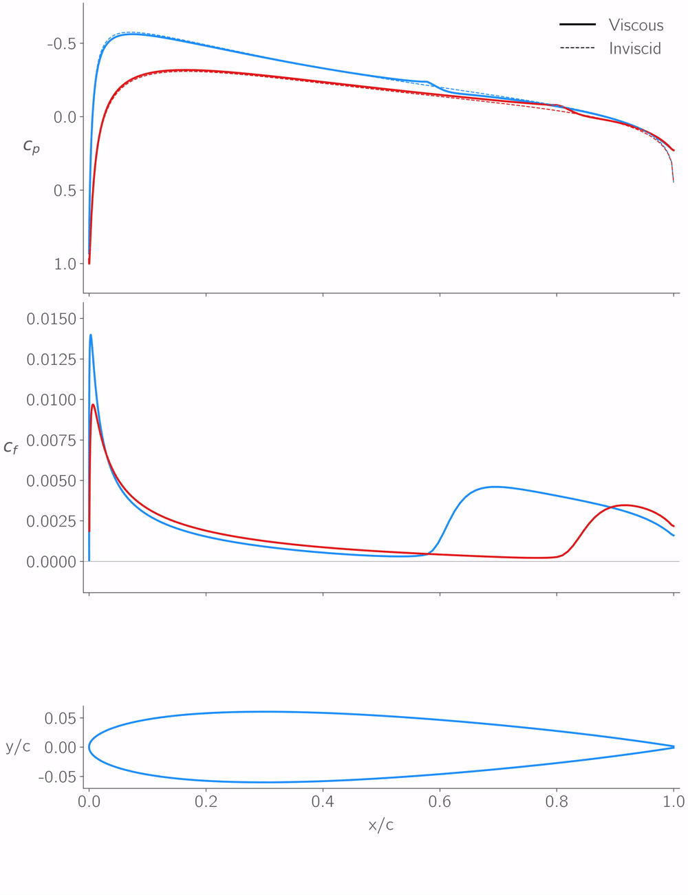
Finally, we save the final figure and use the built-in animation utility to create an optimization movie.
# Save the final figure
CFDSolver.airfoilAxs[1].legend(["Original", "Optimized"], labelcolor="linecolor")
CFDSolver.airfoilFig.savefig(os.path.join(outputDir, "OptFoil.pdf"))

# Animate the optimization
AnimateAirfoilOpt(outputDir, "fc").animate(
    outputFileName=os.path.join(outputDir, "OptFoil"), fps=10, dpi=300, extra_args=["-vcodec", "libx264"]
)
Run it yourself!
To run the script, use the following command:
python single_point.py
In the output directory, it should create the following animation after the optimization completes: